problem09

9. Canon ball.

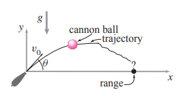
A cannon ball m is launched at angle θ and speed v0. It is acted on by gravity g and a viscous drag with magnitude \(\|c\vec{v}\|\).

1. Find position vs time analytically.
   
2. Find a numerical solution using θ = π/4, \(v_0 = 1\) m/s, g = 1 m/s 2 , m = 1 kg, c = 1 kg/ s.
   
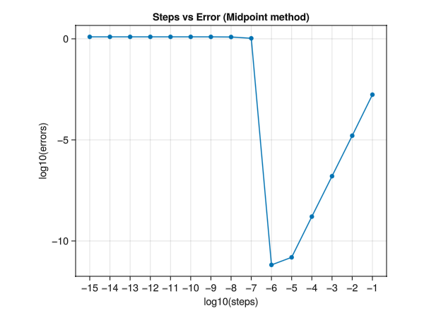
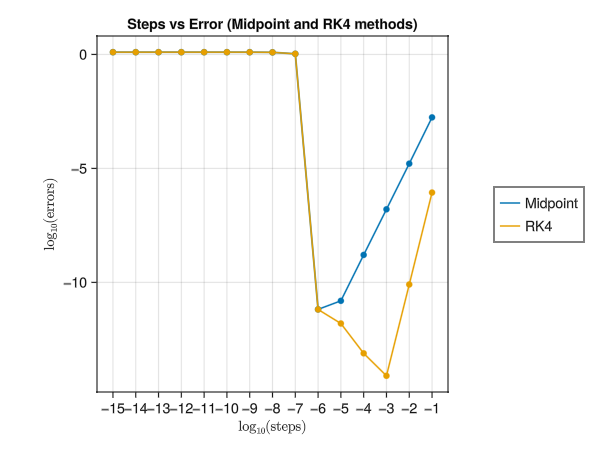
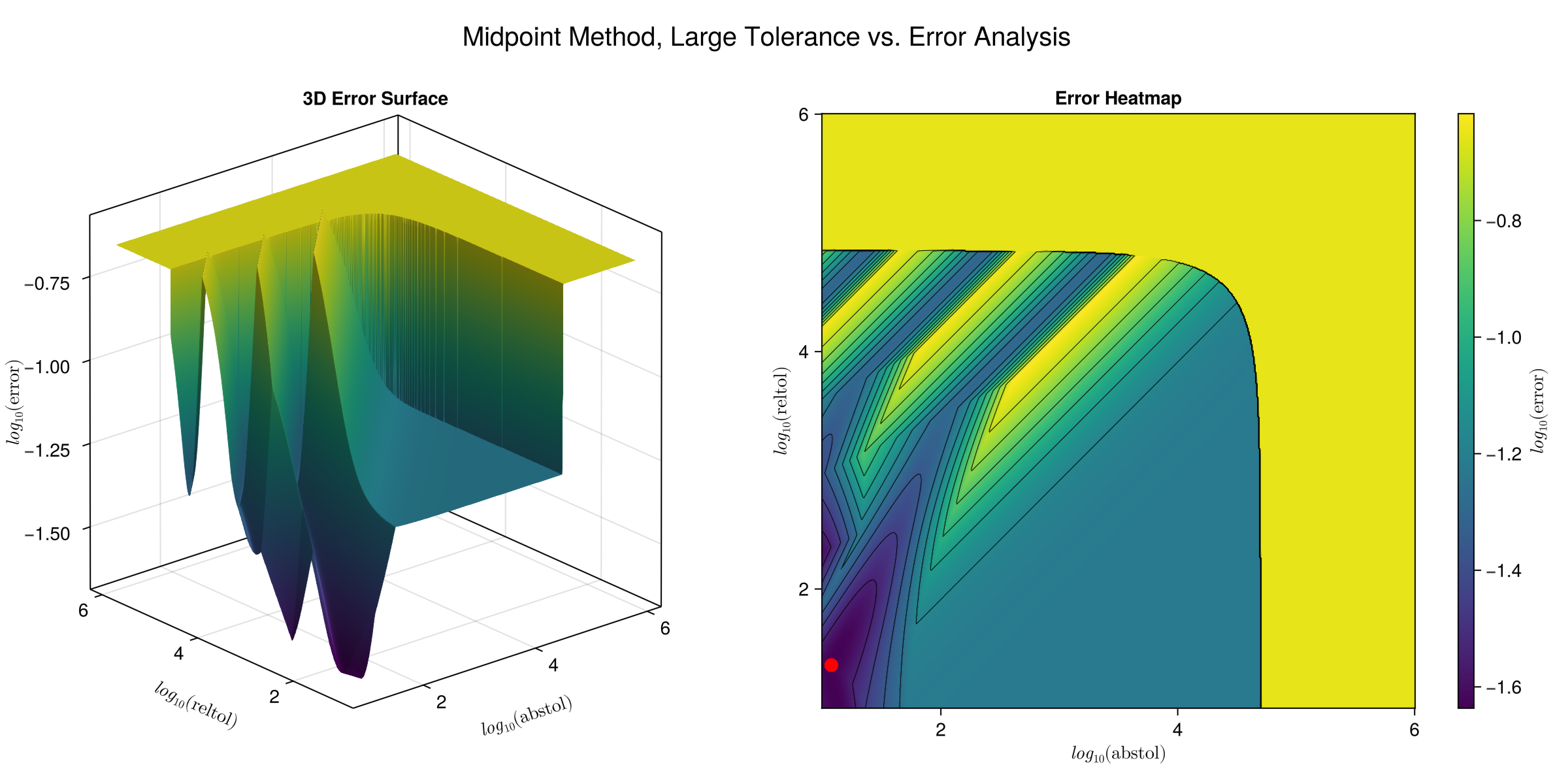
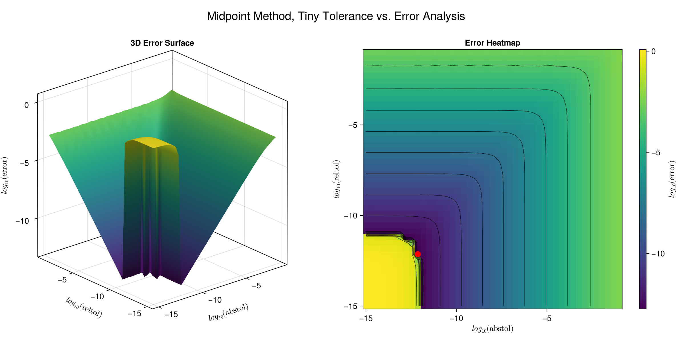
3. Compare the numeric and analytic solutions. At t = 2 how big is the error? How does the error depend on specified tolerances or step sizes?
   
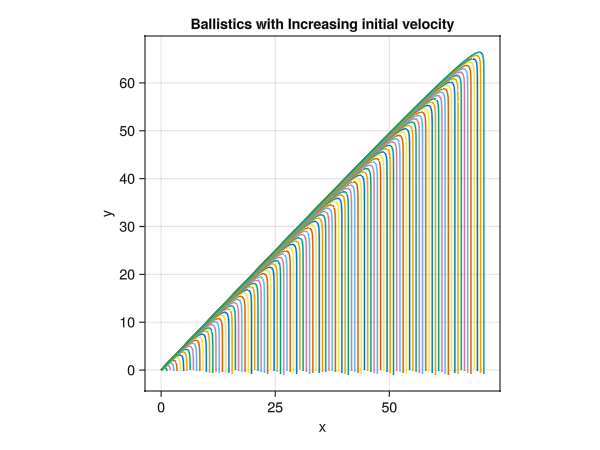
4. Use larger and larger values of v0 and for each trajectory choose a time interval so the canon at least gets back to the ground. Plot the trajectories (using equal scale for the x and y axis. Plot all curves on one plot. As v → ∞ what is the eventual shape? [Hint: the answer is simple and interesting.]
   
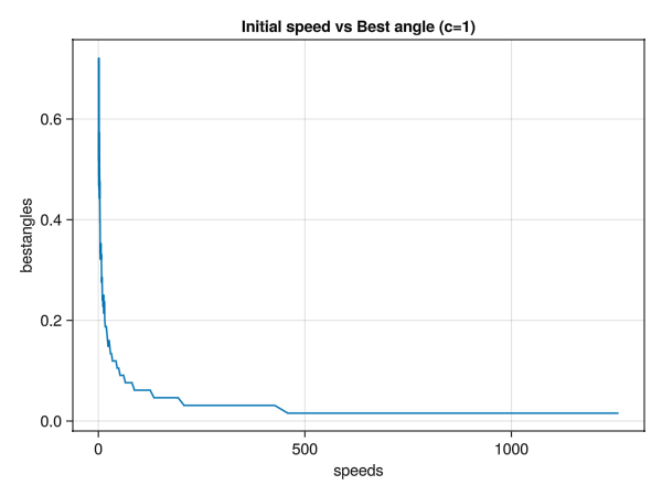
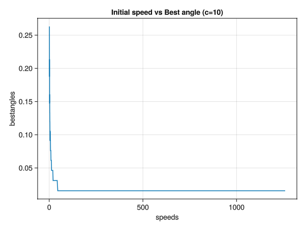
5. For any given v0 there is a best launch angle θ ∗ for maximizing the range. As v0 → ∞ to what angle does θ ∗ tend? Justify your answer as best you can with careful numerics, analytical work, or both.

../../media/problem09/problem09.png

Figure 1: Problem Diagram

1 Find position vs time analytically.

In file ./Ballistics/src/Ballistics.jl:

function analytical_sol(t)
    m, g, c = p.mass, p.gravity, p.viscosity

    u = zeros((4,))
    u[1] = vx0 * (-c/m) * (exp((-c/m)*(t-t0)) - 1)
    u[2] = ((vy0+(m*g/c))*(-c/m)*(exp((-c/m)*(t-t0)) - 1)) + ((-m*g/c)*(t-t0))
    u[3] = (vx0) * (exp((-c/m)*(t-t0)))
    u[4] = ((vy0) + (m*g/c)) * exp((-c/m)*(t-t0)) - (m*g/c)

    return u
end

This turned out to be wrong, it was an integral mistake (integration mistake).

The corrected version in the same file:

function analytical_sol(t)
    m, g, c = p.mass, p.gravity, p.viscosity

    x = x0 + vx0 * ((-m / c) * exp((c / m) * (t0))) * (exp((-c / m) * t) - exp((-c / m) * t0))
    y = y0 + ((vy0 + (m * g / c)) * (-m / c) * (exp((c / m) * t0)) * (exp((-c / m) * t) - exp((-c / m) * t0))) + ((-m * g / c) * (t - t0))
    vx = (vx0) * (exp((-c / m) * (t - t0)))
    vy = ((vy0) + (m * g / c)) * exp((-c / m) * (t - t0)) - (m * g / c)

    u = zeros((4,))
    u[1] = x
    u[2] = y
    u[3] = vx
    u[4] = vy

    return u
end

TODO: Could I have created this analytical solution symbolically?

2 Find a numerical solution using given parameters

In file ./Ballistics/src/Ballistics.jl:

using DifferentialEquations
#...
# problem setup
x0, y0 = 0.0, 0.0
r0 = [x0; y0]
speed0 = 1
launchangle = pi / 4
vx0, vy0 = speed0 * [cos(launchangle); sin(launchangle)]
v0 = [vx0; vy0]
u0 = [r0; v0]

t0 = 0.0
tend = 1.0
tspan = (t0, tend)
p = Parameters.Param(m=1, g=1, c=1)
prob = ODEProblem(Physics.ballistic!, u0, tspan, p)
#...
sol_numeric = solve(prob)
#...
Visualization.plot_trajectory(sol_numeric.u)

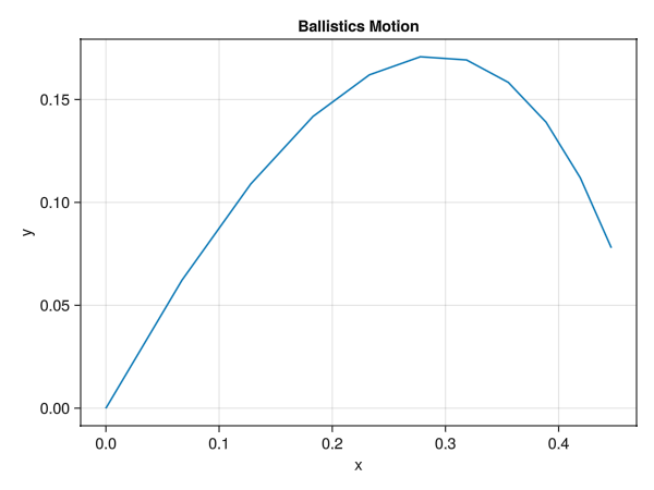
This numerical solution gives the following trajectory:

../../media/problem09/numerical_trajectory.png

Figure 2: System Evolution, Trajectory

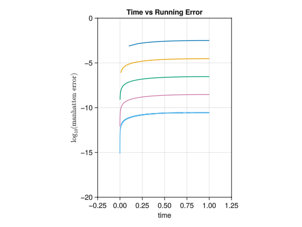
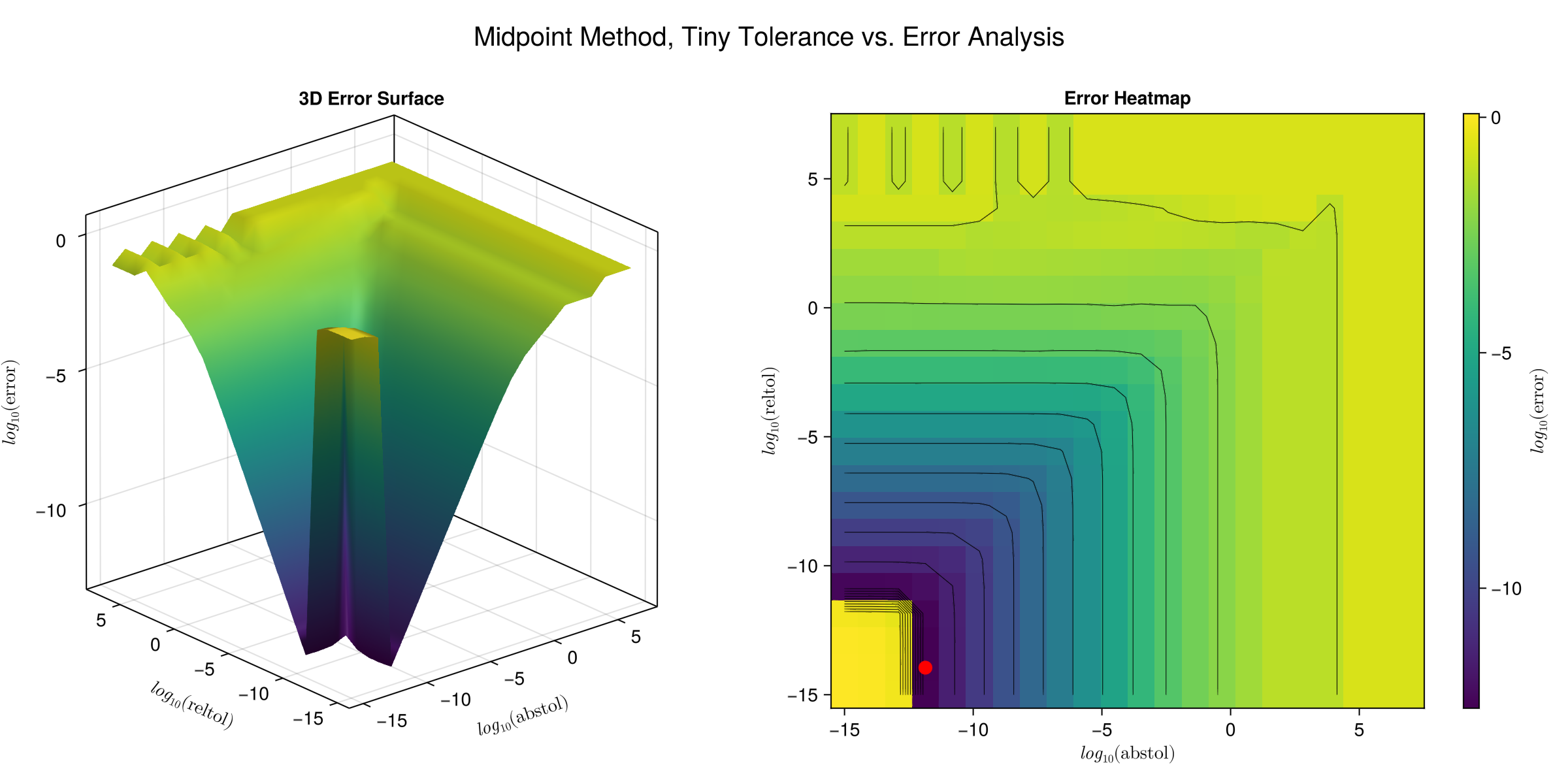
3 Compare the numeric and analytics solutions? Plot time vs error. Plot step size and tolerances vs error.

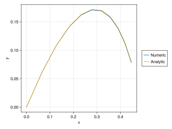
For various initial conditions, the numeric and analytical solutions on the same graph, I was shifting the analytic in x direction by 0.1 unit to be able view both, otherwise they were overlapping with the default tolerances, but then I ended up using a non-dynamic step size explicit solver:

In file ./Ballistics/src/Benchmarks.jl:

module Benchmarks

using DifferentialEquations
using LinearAlgebra

# Abs error for various step sizes
function abs_error_vs_step_sizes(prob, analytical_solve)
    # step_sizes = 10.0 .^ range(-1, -15, step=-1)
    step_sizes = 10.0 .^ range(-1, -5, step=-1)
    abs_errors_midpoint = Vector{Union{Missing, Float64}}(missing, length(step_sizes))
    abs_errors_rk4 = Vector{Union{Missing, Float64}}(missing, length(step_sizes))

    for (i,Δh) in enumerate(step_sizes)
        sol_numeric_midpoint = solve(prob, Midpoint(), dt=Δh, adaptive=false, save_everystep=false)[end]
        sol_numeric_rk4 = solve(prob, RK4(), dt=Δh, adaptive=false, save_everystep=false)[end]
        tend = prob.tspan[2]
        sol_analytic = analytical_solve(tend)

        separation_midpoint = sol_numeric_midpoint - sol_analytic
        separation_rk4 = sol_numeric_rk4 - sol_analytic
        error_midpoint = norm(separation_midpoint)
        error_rk4 = norm(separation_rk4)
    
        abs_errors_midpoint[i] = error_midpoint
        abs_errors_rk4[i] = error_rk4
    end

    log_errors_midpoint = log10.(abs_errors_midpoint)
    log_errors_rk4 = log10.(abs_errors_rk4)
    log_errors_dict = Dict("midpoint"=>log_errors_midpoint, "rk4"=> log_errors_rk4)
    log_steps = log10.(step_sizes)

    return log_steps, log_errors_dict
end

# Abs error for all times
function error_vs_time(prob, analytical_solve)
    N = 5
    step_sizes = 10.0 .^ range(-1, -N, step=-1)
    time_histories = Vector{Union{Missing, Vector{Float64}}}(missing, length(step_sizes))
    error_histories = Vector{Union{Missing, Vector{Float64}}}(missing, length(step_sizes))
    for (i,Δh) in enumerate(step_sizes)
        sol = solve(prob, Midpoint(), dt=Δh, adaptive=false, save_everystep=true)

        timestamps = sol.t
        sol_numeric_midpoint = sol.u
        sol_analytic = analytical_solve.(timestamps)

        separations = sol_numeric_midpoint .- sol_analytic
        manhatten_errors = norm.(separations, Ref(1))
        error_histories[i] = log10.(manhatten_errors)
        time_histories[i] = timestamps
    end
    return time_histories, error_histories
end


end # module Benchmarks

Compare Analytic and Numeric

Time vs Compiled Error, different abstol reltol

Steps Sizes vs Error

Compare Midpoint and RK4

Figure 3: Comparing, Numeric and Analytic Solutions

In file ./Ballistics/src/Benchmarks.jl:

function tolerances_vs_error(prob, analytical_solve)
    N = 15
    error_matrix = Matrix{Float64}(undef, N, N)
    num_granularity = N+7
    abstols = 10.0 .^ range(7, -N, length=num_granularity)
    reltols = 10.0 .^ range(7, -N, length=num_granularity)

    num_samples = length(abstols)*length(reltols)

    xs = Vector{Float64}(undef, num_samples)
    ys = Vector{Float64}(undef, num_samples)
    zs = Vector{Float64}(undef, num_samples)

    for (i, abstol) in enumerate(abstols)
        for (j, reltol) in enumerate(reltols)
            sol_numeric = solve(prob, Midpoint(), adaptive=true, save_everystep=false, abstol=abstol, reltol=reltol)[end]
            sol_analytic = analytical_solve(prob.tspan[2])

            separation = sol_numeric - sol_analytic
            error = norm(separation)
            xs[i+num_granularity*(j-1)] = abstol
            ys[i+num_granularity*(j-1)] = reltol
            zs[i+num_granularity*(j-1)] = error
        end
    end
    xs,ys,zs
end

(did accidentally) Large (>1.0) tolerances

Tiny (<<1.0) tolerances

Both on same plot

Figure 4: Tolerances vs Compiled Eror

Simply put, it seems reducing both abstol and reltol generally reduces error from the analytic solution very quickly. What is the meaning of both is not yet entirely clear.

4 Use larger and larger values of v0, plot all of their trajectory till ball hits ground. What happens to the eventual shape as v -> ∞ ?

In file ./Ballistics/src/Ballistics.jl:

# ...

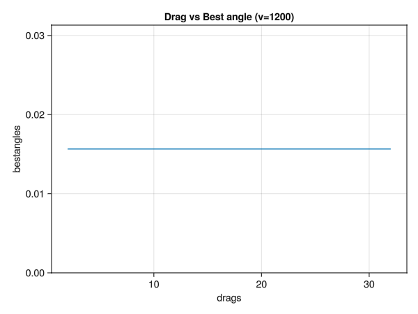
function solve_till_empty(prob)
    conditionatbeggining(u, t, integrator) = t > 0
    removetstop!(integrator) = add_tstop!(integrator, ∞)
    removetstopwhenbeginning = DiscreteCallback(conditionatbeggining,removetstop!)

    condition(u, t, integrator) = u[2] < 0
    affect!(integrator) = terminate!(integrator)
    stopwhenonground = DiscreteCallback(condition, affect!)

    cb = CallbackSet(removetstopwhenbeginning, stopwhenonground)
    sol = solve(prob, RK4(), callback = cb, tstops = [0.1,])

    sol
end

function problem_setup(launchangle, speed0, c)
    x0, y0 = 0.0, 0.0
    r0 = [x0; y0]
    vx0, vy0 = speed0 * [cos(launchangle); sin(launchangle)]
    v0 = [vx0; vy0]
    u0 = [r0; v0]

    t0 = 0.0
    tend = 1.0
    tspan = (t0, tend)
    p = Parameters.Param(m = 1, g = 1, c = c)
    prob = ODEProblem(Physics.ballistic!, u0, tspan, p)
    return prob
end

speeds = range(0, 100)
problems = problem_setup.(Ref(pi/4), speeds, Ref(1))
sols = solve_till_empty.(problems)
Visualization.plot_all_trajectories(sols)

# ...

The plot corresponding to this:

../../media/problem09/initial_velocity_change.png

Figure 5: Increasing intial velocities

5 Plot speed verses best launch angle, numerically or analyticaly or both

I expect 45 degrees to still be consistantly good for launch even with drag.

In file ./Ballistics/src/Benchmarks.jl:

# ...

function best_angle_for_speed(speed0, c)
    launchangles = pi/4 .* ((range(-1.0, 1.0, 300)) .^ 3.0 .+ 1.0)

    max_range = 0
    argmax_theta = 0
    for launchangle in launchangles
        # problem setup
        prob = problem_setup(launchangle, speed0, c)

        sol = solve_till_empty(prob)
        cur_range = sol.u[end][1]
        if cur_range > max_range
            max_range = cur_range
            argmax_theta = launchangle
        end
    end
    argmax_theta
end

speeds = 10.0 .^ range(0.0, 3.1, 100)
bestangles = []
for speed0 in speeds
    bestangle = best_angle_for_speed(speed0, 1)
    push!(bestangles, bestangle)
end
Visualization.plot_best_angle_for_speeds(speeds, bestangles)

# ...

The weird choice for launchangles is for concentrating numeric choices for launchangles near \(\pi \over 4\). This produces:

../../media/problem09/speed_vs_bestangle_c_1.png

../../media/problem09/speed_vs_bestangle_c_10.png

Figure 6: Best Angles for initial speeds

It seems that my intuition was way off. It seems the best angle quickly becomes closer to zero as the initial velocity increases.

In file ./Ballistics/src/Ballistics.jl:

speed0 = 1200.0
bestangles = []
drags = 2.0 .^ range(1.0, 5.0)
for c in drags
    bestangle = best_angle_for_speed(speed0, c)
    push!(bestangles, bestangle)
end
Visualization.plot_best_angle_vs_drag(drags, bestangles)

TODO: There isn’t much change in the eventual best angle for large velocities as drag changes. It does not seem right, but the best angle in such case seems to be some constant close to zero. I will explore this more later. The plot generated by above code is:

../../media/problem09/best_angle_vs_drag.png

Figure 7: Drag vs best angle (v = 1200)

This concludes my attempt of problem09.