problem12

12. Canon ball 2.

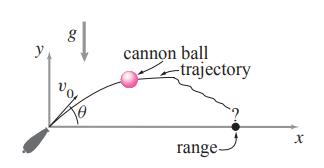
A cannon ball \(m\) is launched at angle \(\theta\) and speed \(v_0\). It is acted on by gravity \(g\) and a quadratic drag with magnitude \(\|cv^2\|\).

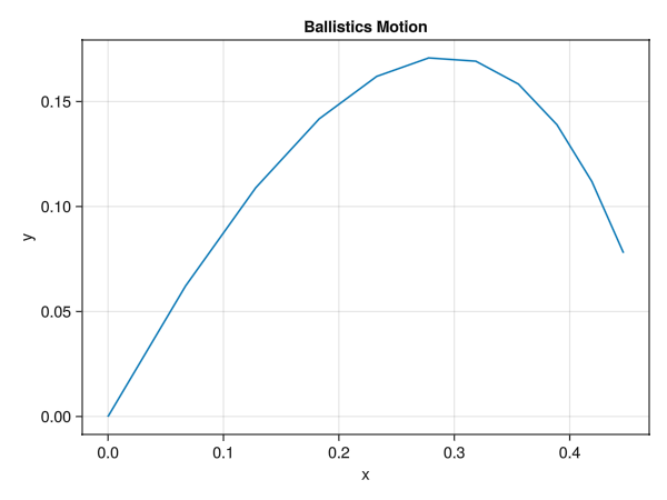
1. Find a numerical solution using \(\theta = \pi/4\), \(v_0 = 1\) m/s, \(g = 1\) m/s\(^2\), \(m = 1\) kg.
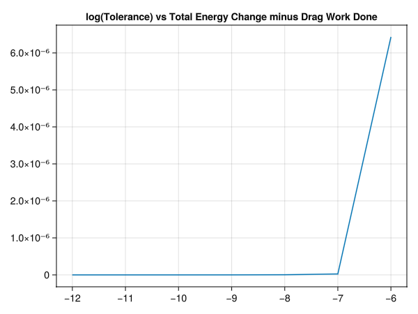
2. Numerically calculate (by integrating \(\dot{W} = P\) along with the state variables) the work done by the drag force. Compare this with the change of the total energy. Make a plot showing that the difference between the two goes to zero as the integration gets more and more accurate.

../../media/problem12/problem12-ballistic.png

Figure 1: External Forces on System

1 Find a numerical solution using \(\theta = \pi/4\), \(v_0 = 1\) m/s, \(g = 1\) m/s\(^2\), \(m = 1\) kg.

Same as in problem09

../../media/problem09/numerical_trajectory.png

Figure 2: System Evolution, Trajectory

2 Numerically calculate (by integrating \(\dot{W} = P\) along with the state variables) the work done by the drag force. Compare this with the change of the total energy. Make a plot showing that the difference between the two goes to zero as the integration gets more and more accurate.

I take this oppurtunity to implement the ‘slither’ for trajectory similarity, that was introduced

In file ./BallisticDrag/src/BallisticDrag.jl:

module BallisticDrag

import DifferentialEquations
import LinearAlgebra
import GLMakie

@kwdef struct Parameters
    m::Float64
    g::Float64
    c::Float64
end

function myode!(du, u, p, t)
    r = u[1:2]
    v = u[3:4]
    vcap = v / LinearAlgebra.norm(v)

    j = [0;1]
    gravity = (p.m*p.g)*(-j)
    drag = abs(p.c*LinearAlgebra.dot(v, v))*(-vcap)
    F = gravity+drag
    a = F / p.m

    drag_power = LinearAlgebra.dot(drag, v)

    du[1:2] = v
    du[3:4] = a
    du[5] = drag_power
end

p = Parameters((global m=1), (global g=1), (global c=1))
tspan = (0.0, (global tend=10.0))
u0 = [0.0;0.0;10.0;10.0;0.0]
odeprob = DifferentialEquations.ODEProblem(myode!, u0, tspan, p)

function tae_diff(tolerance)
    sol = (DifferentialEquations.solve(odeprob; abstol=tolerance, reltol=tolerance))
    tpoints = length(sol.t)

    sol = reduce(hcat, sol.u)'

    work = sol[:, 5]
    work_change = work[2:end] .- work[1:end-1]

    v = sol[:, 3:4]
    kinetic = (1/2)*(m)*([LinearAlgebra.dot(v[i, :], v[i, :]) for i in 1:size(v, 1)])
    y = sol[:, 2]
    potential = (m*g)*y
    total = kinetic .+ potential
    change = total[2:end] .- total[1:end-1]

    return sum(abs.(change .- work_change)) # / tpoints
end

# Plot (energy - workdone) TAE (total absolute error) with increasing accuracies
powers = -range(6, 12)
tolerances = 10.0.^powers
tae_energy_change = tae_diff.(tolerances)

fig = GLMakie.Figure()
ax = GLMakie.Axis(fig[1,1], title="log(Tolerance) vs Total Energy Change minus Drag Work Done")
GLMakie.lines!(ax, powers, tae_energy_change)
GLMakie.save("tolerances_vs_total_energy_change_minus_drag_work_done.png", fig)
GLMakie.display(fig)

end # module BallisticDrag

This produces:

../../media/problem12/tolerances_vs_total_energy_change_minus_drag_work_done.png

Figure 3: Tolerances vs Total Energy minus Drag work done

This concludes my attempt of problem12.